Lead PI: Chrys Chryssostomidis
Funding Period: 2/2019 – 1/2021
Project number: 2019-R/RC-150
Strategic Focus Area: Healthy Coastal Ecosystems, Sustainable Fisheries and Aquaculture
WHAT IS MULTI-FIDELITY MODELING?
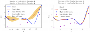
The multi-fidelity model is a data-driven model that combines the low-fidelity (LF) and high-fidelity (HF) measurements in a probabilistically principled manner. It learns and exploits the correlations between the LF and HF measurements. The presented multi-fidelity model is based on Gaussian process regression (GPR) – a machine learning model that learns functions from data. GPR has two distinct characteristics: (1) GPR is a non-parametric regression model. This is in contrast to parametric regression models where the form of the regression model must be determined before learning the parameters, for example linear regression. (2) GPR is a probabilistic regression model that yields the prediction and the uncertainty associated with the prediction. The uncertainty provides an estimate of the trustworthiness of the multi-fidelity predictions and can be used to guide new samples. For example the new high-fidelity samples can be acquired at points that have high uncertainty. This is useful for effective allocation of data acquisition resources.
WHO CAN USE MULTI-FIDELITY MODELING?
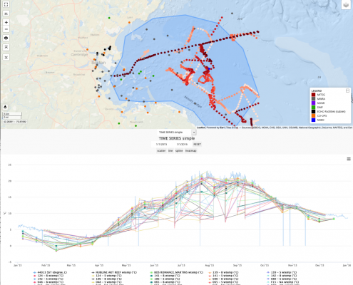
For many applications HF data are costly to obtain, while LF data are relatively cheap to acquire. For example, for estimating sea surface temperature (SST) in a region of interest, we may be able to deploy buoys with high precision sensors to few locations in the region of interest and once a month. Each measurement is an HF data point. Clearly, the number of HF data points is limited by the scares resources that are available and we may not have enough HF measurements needed to build desirable spatio-temporal SST maps. On the other hand, we may be able to obtain many less accurate SST measurements relatively cheaply. For example, we can obtain SST measurements from a variety of satellites. The satellite SST measurements are available at a much higher spatial resolution than few buoys deployed in a large region and the satellites also have much better temporal resolution, i.e. daily, than monthly buoy measurements. However, satellite measurements are not accurate and require calibration. In this example, the buoy measurements are few but accurate and can serve as the HF measurements and satellite measurements are many but prone to errors. In scenarios such as this example, it has been shown that the multi-fidelity model can produce results with few HF measurements and many LF measurements that are as accurate as the regression model with many HF measurements. In other words, the multi-fidelity model compensates for the insufficiency of the HF measurements by utilizing the LF measurements. If your application fits the few-but-accurate HF measurements and many-but-inaccurate LF measurements you may benefit from using the presented multi-fidelity modeling.
HOW TO USE THE MULTI-FIDELITY MODEL?
USE ONLINE! coming soon
The multi-fidelity model is developed in MATLAB and can be used freely. The code can be downloaded from GitHub via https://github.com/hbabaee/MFSST. The instruction to use the code is as follows. The LF and HF data must be provided to the code in the following format:
LF.X: This is the coordinates of the input space and it is an array of size N_L by d, where N_L is the number of low-fidelity measurements and d is the dimension of the input space. For example, in the case of spatio-temporal SST model, the input space is (Latitude, Longitude, Time). Therefore, LF.X has three columns (d=3) corresponding to three-dimensional input space. Please see https://github.com/hbabaee/MFSST/tree/master/Spatio-Temporal as an example of spatio-temporal SST model.
LF.Y: This is the LF measurement of the target function, i.e. the quantity of interest (QoI) and it is a vector of size N_L by 1. Each row of the vector LF.Y must be the value of QoI measured at the corresponding row of the array LF.X.
HF.X: Similar to LF.X points, HF.X encompasses the coordinates of the input space and it is an array of size N_H by d, where N_H is the number of HF measurements and d is the dimension of the input space.
HF.Y: This is also analogous to LF.Y. HF.Y encompasses the HF measurement of the target function and it is a vector of size N_H by 1.
Once the multi-fidelity model is trained, it can be used for predictions at new points via the function predictor_f_H(X), where X is an array of size Np by d, where Np is the number of prediction points, and d is the dimension of the input space.
CODE REPOSITORIES
This section uses a plugin to provide dynamic updates to linked code repositories on Github.
CONTRIBUTORS
PROJECT DATA
This section should list direct links to sites where project data can be EASILY accessed.
Examples:
- http://mseas.mit.edu
- http://ifcb-data.whoi.edu
- http://www2.neracoos.org/datatools/data_access/THREDDS
- https://www.bco-dmo.org/project/529583
- http://uhslc.soest.hawaii.edu
- http://www.ncdc.noaa.gov/data-access/paleoclimatology-data/datasets
- OPeNDAP
- http://www.rvdata.us/catalog/
- http://www.nodc.noaa.gov
- http://ocb.whoi.edu
- https://www.ncei.noaa.gov
- http://www.neracoos.org/necan
- SOS (Sensor Observation Service) web service.
and many more…
HIGHLIGHTS | Explanded Project
 https://seagrant.mit.edu/wp-content/uploads/2025/06/SeaGrant_Support_Map_6_2_2025.png
845
1688
Lily Keyes
https://seagrant.mit.edu/wp-content/uploads/2023/05/MITSG_logo_website.png
Lily Keyes2025-06-03 13:51:562025-06-03 13:57:29Sea Grant Support: A Note from the Director
https://seagrant.mit.edu/wp-content/uploads/2025/06/SeaGrant_Support_Map_6_2_2025.png
845
1688
Lily Keyes
https://seagrant.mit.edu/wp-content/uploads/2023/05/MITSG_logo_website.png
Lily Keyes2025-06-03 13:51:562025-06-03 13:57:29Sea Grant Support: A Note from the Director https://seagrant.mit.edu/wp-content/uploads/2025/03/MaritimeConstortium2.jpg
600
900
Lily Keyes
https://seagrant.mit.edu/wp-content/uploads/2023/05/MITSG_logo_website.png
Lily Keyes2025-03-26 12:40:252025-03-26 12:52:11MIT Maritime Consortium Sets Sail
https://seagrant.mit.edu/wp-content/uploads/2025/03/MaritimeConstortium2.jpg
600
900
Lily Keyes
https://seagrant.mit.edu/wp-content/uploads/2023/05/MITSG_logo_website.png
Lily Keyes2025-03-26 12:40:252025-03-26 12:52:11MIT Maritime Consortium Sets Sail https://seagrant.mit.edu/wp-content/uploads/2021/03/OceanEnergies.jpg
1440
1920
Lily Keyes
https://seagrant.mit.edu/wp-content/uploads/2023/05/MITSG_logo_website.png
Lily Keyes2025-01-21 09:44:222025-02-25 10:09:21Now Accepting Preproposals: FY2026-2028 Core RFP
https://seagrant.mit.edu/wp-content/uploads/2021/03/OceanEnergies.jpg
1440
1920
Lily Keyes
https://seagrant.mit.edu/wp-content/uploads/2023/05/MITSG_logo_website.png
Lily Keyes2025-01-21 09:44:222025-02-25 10:09:21Now Accepting Preproposals: FY2026-2028 Core RFP